

Principal component analysis (PCA) attempts to find true trends hidden in complex data by filtering out noise and redundancy. It does this by treating complex data as a n-dimensional shape (where n is the number of measurements in your study) and fitting that shape to n 1-dimensional lines called: “principal components” and ranking these lines by the percentage of data variation that they capture.
For example, if your research question is “How many factors determine American’s opinions on Wall Street?” you might design a questionnaire with 3 questions (10-pt scale questions) and survey 25 people (see figure above). When you plot this data in 3-dimensions, you will see that your data will look like a 3-dimensional shape. Applying PCA, you’ll find that a single 1-dimensional line captures 90% of the variability in the data. This allows you to form and test hypotheses what “one-factor” most determines peoples “Wall Street opinions”. In this example here, “principal component 1 (PC1)” or the “top-ranked 1-dimensional fit line” is meant to reflect the American 2-party political spectrum.
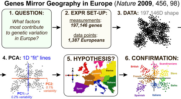
A recent paper in Nature answered the question: “What factors most contribute to genetic variation in Europe?” by using PCA to analyze 197,146 genes of 1,387 Europeans. By plotting only the top two 1-dimensional fit lines (PC1 and PC2) they were able to reduce the problem from a 197,146-dimensional shape to a 2-dimensional shape. By examine the geometry of this shape, they found that PC1 and PC2 roughly corresponded to the North/South and East/West axes of Europe, and thus that the geography of Europe is the top-ranked determinant of the genetic variation of Europeans.
Overall, these examples are meant to illustrate how, when you don’t know the answer to your question, you often take many more measurements than you need to. PCA helps you reduce the dimensionality of your data to ranked principal components that represent underlying “drivers of variability.” The identity of these drivers can be confirmed by examing common factors of sub-groupings at the extremes of each principal component (e.g. for example 1, republicans cluster at one extreme while democrats cluster at another extreme).
Ever since the human genome was sequenced, biomedical scientists have lived and worked in an era of “big data.” Unfortunately, sometimes knowing “everything” is the same as knowing “nothing” as the answer to your specific research question is buried in pages and pages of irrelevant data. PCA is a valuable tool to help researchers find their “needle” in today’s big data “haystack.”
REFERENCES:
- Long, J.D. PRINCIPAL COMPONENT ANALYSIS (PCA) VS ORDINARY LEAST SQUARES (OLS): A VISUAL EXPLANATION, CerebralMastication.com, 2010
- Ringner, M. What is Principal Component Analysis? Nature Biotechnology, 2008, 26, 303-304.
- Shlens, J. A tutorial on principal component analysis. arXiv preprint arXiv:1404.1100, 2014.
- Smith, L. I. A tutorial on principal components analysis, Technical report, Cornell University, USA 2002.
- Novembre, J.; Johnson, T.; Bryc, K.; Kutalik, Z.; Boyko, A.R.; Auton, A.; Indap, A. King, K.S.; Bergmann, S.; Nelson, M.R.; Stephens, M.; Bustamante, C.D. Genes mirror geography within Europe. Nature, 2008, 456, 98-101

This work by Eugene Douglass and Chad Miller is licensed under a Creative Commons Attribution-NonCommercial-ShareAlike 3.0 Unported License.