Category Archives: Biology

Understanding the Diffraction Limit in Microscopy

microscopy-defraction-limit-v4

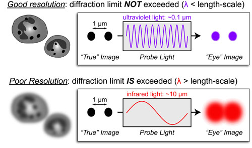
Basic light microscopy can only resolve objects that are larger than 100 nm which means that while it can visualize animal cells (~10,000nm), organelles and bacteria (~1,000nm), it cannot visualize viruses (<100nm), proteins (<10nm) or small molecules(~1nm) (see post summarizing Biological Scales). This limitation is known as the “diffraction limit” and is caused by the fact light only interacts differently with objects separated by more than one wavelength (λ). Intuitively, its helpful to think of each of these wavelengths as “a minimum pixel size” for a computer image where: infrared light (λ ~ 10.0μm) has pixels 100 times larger than ultraviolet light (λ ~ 0.1μm).

Continue reading

Introduction to ELISA

sandwich-elisa-intro-v6

ELISA or Enzyme-Linked Immunosorbent assay is the most commonly used method for measuring proteins concentrations in solution. It is extensively used both in the laboratory (e.g. culture supernatant) and the clinic (e.g. blood tests) due to its simplicity and adaptability to other protein-based assays such as high throughput screening. The way it works is outlined in the figure above and described in detail below:

Continue reading

Introduction to Flow Cytometry

Web

Flow cytometry is a technique that can quantitatively measure (1) protein expression levels per single cell and (2) amounts of different cell-types (based on a protein-maker) for thousands of cells in minutes! Flow cytometers use hydrodynamic focusing to force a mixture of stained cells into a single-file line through a flow cell. Then, each cell, sequentially, passes through a laser beam which excites the fluorophore allowing quantification of protein expression for all proteins that are stained!

Continue reading

Hybridomas for Large-scale Antibody Production

antibody-production-v3

Following up on our post introducing antibody-based experiments, we wanted to describe how antibodies are made in large volume: First, an animal is immunized with the protein (or peptide) of interest; Second, the spleen is dissected and the plasma cells producing the antibodies of interested are isolated; Finally, these plasma cells are fused with myeloma cells to “immortalize” them into a hybridoma (an antibody-producing cell-line that can be cultured indefinitely).

Continue reading

Introduction to Antibody Based Experiments

Web

Antibodies are immune proteins that can be easily engineered to bind (and “detect”) any given protein in via a simple vaccination method. To “signal” the presence of detected proteins, fluorophores are attached to “stain” the protein (and cell or tissue expressing it) a particular color. These fluorescent probes, have been utilized to identify the location of specific proteins in tissue sections (histology), single cells (microscopy) and quantify the amount of protein in cells (flow cytometry) and in complex mixtures (western blotting).

Continue reading

Back-crossing mutant mice into a genetic background

Web

Inbred mouse lines are used for most laboratory mouse work to make sure that all the mice have nearly identical genetic backgrounds (i.e. genetic code). These lines were originally generated by repeatedly mating mice with their siblings which minimized genetic variability and makes these mice as close to clones of each other as is practically possible.

Continue reading

Introduction to Mouse Breeding

mouse-breeding-summary-v2

Careful breeding/husbandry of mice is important when one is asking genetic questions about disease. Such questions include: “Does gene X contribute to cancer?”, “Does my drug treat cancer by targeting gene X?”.

In general, these questions can only be answered by comparing mice that have gene X (WT or +/+) or don’t have gene X (KO or -/-). To make sure the genetic difference is the only difference between the mice, you usually compare siblings of inbred mouse-lines which have the same sex, age, environment and genetic background.

Continue reading

What is Principal Component Analysis??

FIG1-PCA-intuition-v5-op

Principal component analysis (PCA) attempts to find true trends hidden in complex data by filtering out noise and redundancy. It does this by treating complex data as a n-dimensional shape (where n is the number of measurements in your study) and fitting that shape to n 1-dimensional lines called: “principal components” and ranking these lines by the percentage of data variation that they capture.

Continue reading

A “Chemical-Structure Map” of the Metabolome

global-metabolism-v7

I’ve always struggled to connect the structures of natural products with the biosynthetic pathways that generate them. I recently found a great resource in the Kyoto Encyclopedia of Genes and Genomes (KEGG) which helped me address this problem directly. The figure above is an adaptation of several of their pathway charts most especially that pictured here.

Continue reading

An Idea for Visualizing Receptor/Ligand X-Ray Structures

Web

As an organic chemist, I have always had difficulty relating the 3D PDB/X-ray structures of receptor/ligand complexes to the 2D chemical drawing chemist build their “chemical insight” off of. In the figure above, I present an idea to bridge the gap by presenting sets of receptor residues as “surfaces” interacting with the two types of 2D representations chemists use to think about chemistry.

Continue reading

Estimating Metabolite Concentrations at Steady State

Biosynthetic Pathway-Funnel Analogy

In a follow up to our post on sequential biochemical pathways, we next wanted to present an method to approximate the concentration of a metabolic intermediate in a biosynthetic pathway. In general, under steady state conditions, the steady state concentration of a metabolite can be estimated from the ratio of the Vmax for the upstream rate-determining enzyme over the rate of decay of that metabolite. A more complete equation is detailed below and further discussed in our post on Estimating Protein/Metabolite Levels from RNAseq data.

Continue reading

Kinetics #3: Branch Points in Biochemical Pathways

catalysis-kinetics-intuition-v6

In a follow up to our posts on Intuiting Enzyme Kinetics and Sequential Biochemical Pathways, we next wanted to consider the kinetic curves branch points in biochemical pathways (or equivalently kinetic competitions). Luckily exact mathematical models exist for competitive first-order processes (see below) and we can use these to develop intuitive rules (figure above) if we consider these pathways to be approximately pseudo-first order (which is often true in the context of biosynthetic pathways).

Continue reading

Kinetics #2: Sequential Biochemical Pathways

catalysis-kinetics-intuition-v6

In a follow up to our post our post on intuiting enzyme kinetics, we next wanted to consider the kinetic curves for sequential biochemical pathways. Luckily exact mathematical models exist for sequential first-order processes (see below) and we can use these to develop intuitive rules (figure above) if we consider these pathways to be approximately pseudo-first order (which is often true in the context of biosynthetic pathways).

Continue reading

Kinetics #1: Catalyzed Reaction Timescales

Kinetic-Thermodynamic Models Overview-v1

Most chemical and biochemical research concerns reaction that are catalyzed by either an enzyme or a chemical catalyst. Unfortunately, when we learn chemical kinetics, it is usually in the context of idealized: uncatalyzed 0th-order, 1st-order of 2nd-order chemical reactions. Luckily the intuition we learn from 0 and 1st order processes can be readily extended to catalyzed processes by invoking the pseuso-1st order approximation. Below we describe how to “think about” the most common enzymatic/catalytic kinetic curves you may encounter.

Continue reading

Binding #3: Competitive Inhibition

Kinetic-Thermodynamic Models Overview-v1

While many drugs act like agonists and “turn on” their target/receptor (see posts on Hill Equation and Agonist Limits), many more drugs act like antagonists and “turn off” their target/receptor. One of the most common mechanisms by which drugs “turn off” a target receptor (R) is by blocking the binding of its natural ligand (L). This mechanism is called competitive inhibition and the antagonist is known as an inhibitor (I). Here there are two dissociation constants:the Kd which describes the strength of the interaction between R and L and the Ki which describes the strength of the interaction between R and I.

Continue reading